
When I started my postdoc in 1998, I think it is safe to say that the Holy Grail (or maybe Rosetta Stone) for many evolutionary biologists was a concept called the Adaptive Landscape. The reason for such exalted status is that the adaptive landscape was then – and remains – the only formal quantitative way to predict and interpret an adaptive radiation of few organisms into many. I was heavily indoctrinated into this framework - as my postdoc was at UBC during precisely the time when Dolph Schluter was writing his now-classic book The Ecology of Adaptive Radiation.
Adaptive landscapes come in several forms (e.g., genotype
based, allele frequency based, phenotype based), and the one we are concerned
with here is the “phenotypic adaptive landscape.” Perhaps the first serious description
of this landscape was the one presented by George Gaylord Simpson in his 1953
book The Major Features of Evolution. In essence, Simpson’s landscape
depicts phenotype combinations (e.g., population average values for two
important traits, such as beak size and beak shape for birds) and the expected
fitness associated with a population having those mean values. The resulting
landscapes are expected to be “rugged,” with various peaks of high fitness
separated by valleys of low fitness. The idea is that a lineage (e.g., of
birds) is expected to diversify phenotypically into multiple species that each occupy
one of those different high-fitness peaks, with few individuals having
phenotypes in the low-fitness combinations between the peaks. From one species
thus comes many in a predictable way by different species matching their traits
to particular resources or habitats that represent high-fitness peaks on the adaptive
landscape,
This adaptive landscape idea remained largely conceptual, or
heuristic, until Lande (1976, 1979) figured out how to represent it mathematically. Then
a bit later, Lande and Arnold (1983) showed how to link the adaptive landscape to
formal estimates of natural selection at the phenotypic level – thus providing a
means for formally estimate the landscape. This theoretical work spurred
several decades of intense interest in attempting to quantify adaptive
landscapes – or parts of them – for particular adaptive radiations. Yet the
effort required turned out to be rather extreme for several reasons. Most critically,
perhaps, the full landscape can be specified only if one knows the fitness of
individuals across the entire range of phenotypic space (e.g., from small beaks
to large beaks for every possible beak shape value from pointy to blunt). Yet,
almost by definition, individuals with phenotypes of low fitness should be rare
in nature - because they are constantly
selected against; and so the fitness of phenotypes between species tend to be
unknown in nature.
The Holy Grail
Owing to this problem of “missing phenotypes,” as well as
other difficulties, I would argue that no formal adaptive landscape – in the Lande
sense – existed for any natural radiation of organisms at the time I started my
postdoc. Yet its predictive promise made it the Holy Grail of the time.
Although no adaptive landscapes had been formally estimated,
some studies got part way there (see the Appendix below on “other landscapes I have
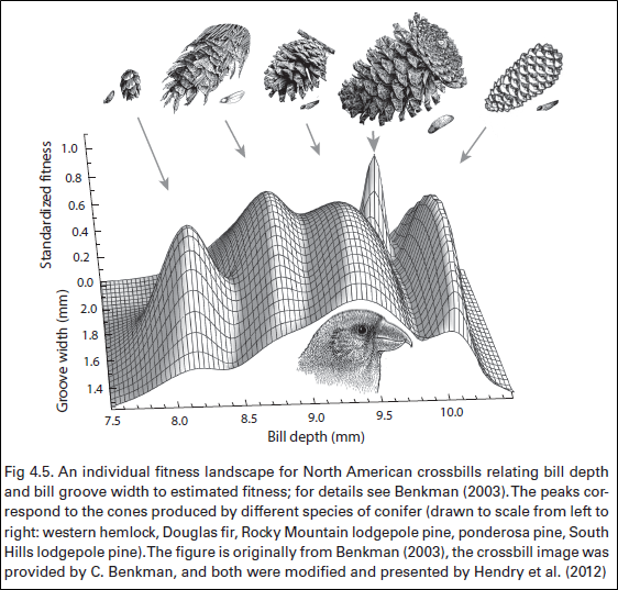
known and loved”). As one example, Benkman (2003) measured the performance of
crossbills on different types of conifer cones and used these estimates and
other information to construct an “individual fitness landscape” spanning the
range of phenotypes – that is, the expected fitness of an individual having each
possible combination of beak trait values. As had been predicted, the landscape
had peaks of high fitness near the average phenotypes of the different
crossbill types – and those peaks were separated by phenotypes with low fitness
– yet something was missing.
 |
| This figure is from my 2017 book. |
In particular, a formal adaptive landscape relates MEAN phenotypes for a population (assuming a particular phenotypic variance) to the expected MEAN fitness of that population, which requires a particular conversion – as the gif below (made by Marc-Olivier Beausoleil) illustrates. When this conversion takes place, the fitness peaks tend to sink and the fitness valleys tend to rise – because the adaptive landscape averages fitness across all of the phenotypes in a population, which inevitably span a range of fitnesses on either side of a peak (or valley). That is, because a population adapted to a fitness peak will have some variation in phenotypes, the off-peak individuals will reduce mean population fitness relative to a population where all individuals were identical and had phenotypes EXACTLY on the peak. The inevitable is that adaptive landscapes based on population means are always smoother than those based on individual fitness values. As an example, the individual fitness peaks for crossbills shown above tend to disappear if converted to a formal adaptive landscape based on population means (C. Benkman pers. comm.)

So, as time went on, a formal adaptive landscape for an adaptive
radiation in nature remained elusive.
My Galapagos Dreams
In 2002, I had the opportunity to visit Galapagos at the
behest of Jeff Podos (UMASS Amherst) who had just received an NSF Career Grant
that could fund my participation. I was really excited and read all of the
classic books by Lack (1947), Bowman (1961), and Grant (1998). Yet, I still had
no real practical experience with Galapagos or even with bird research. Thus,
on my first visit, I decided to not actually conduct any of my own research but
rather learn about the system – both by helping Jeff with his research and also
simply walking around in the field making natural history observations that
might motivate future experiments. A highlight from that year was the afternoon
I spent in the field with the deacons of all things finch, Peter and Rosemary
Grant.

One of the major efforts of Jeff’s team was to capture finches at a focal site (El Garrapatero), measure their beak traits, band them, and then relate those traits to song features and mating. Within a year, I had encouraged an increasing emphasis on using the banded birds to track inter-annual survival. When it was clear that this effort would be productive, I set the goal of – once and for all – estimating the adaptive landscape – in the formal way – for Darwin’s finches at this site.

My first step in this effort was to use the extremely-variable population of Geospiza fortis (the medium ground finch) at El Garrapatero to measure selection across their phenotypic distribution. This population had long been suggested to be bimodal in its beak size distribution, with somewhat distinct “large” and “small” beak morphs. My idea was that the fitness landscape should show a valley between the two morphs, such that intermediate birds have lower fitness – a selective function called disruptive selection. Using two years of data, low-and-behold, disruptive selection between the beak modes (and stabilizing selection around each mode) is what we found. This initial discovery was exhilarating but (1) we had only two years of data, (2) we had a potentially imprecise measure of fitness (survival over one year), and (3) we were looking at only one species.
 |
| This figure is from my 2017 book. |
It took another 10 years of accumulated data – contributed by many team members and collaborators working at El Garrapatero – to solve the first of those problems. In particular, Marc-Olivier Beausoleil (graduate student of Rowan Barrett at McGill) was able to compile years of the most intensive data collection for G. fortis to show that, yes, disruptive selection was always working to maintain some separation of the two morphs (large and small) – and that the intensity of this selection could be explained by weather conditions. Specifically, disruptive selection was strongest when dry periods followed wet periods – probably because many fledglings were produced during wet periods which then increased competition (and hence mortality) during subsequent dry periods.

But these landscapes were still at the level of the individual (rather than population mean), and they still showed only one species, whereas the Geospiza radiation at this location has four species: the small ground finch (Geospiza fuliginosa), the medium ground finch (Geospiza fortis), the large ground finch (Geospiza magnirostris), and the cactus finch (Geospiza scandens). When would we have enough data for this more comprehensive effort.
After 17 years of data collection that included more than 3400
individual birds, we set out to give it a try. For a fitness surrogate, we
chose longevity, which Peter and Rosemary had previously shown was strongly
correlated with total fitness (note: we could not track reproductive output,
such as the number of fledglings, in our population). Marc-Olivier Beausoleil
led this effort and first calculated an individual fitness landscape, relating
the fitness of individual birds to their individual phenotypes across the
entire dataset. As expected, and as shown in other studies (crossbills, African
seedcrackers, and more – see Appendix), the individual fitness landscape was
rugged, showing clear peaks and valleys. Further, the average phenotypes of each
species (and the two morphs of G. fortis) were situated fairly close –
in phenotypic space – to the estimated peaks of high fitness.
Would this reasonable and logical landscape hold up when the
individual fitness landscape was converted to a formal population mean adaptive
landscape. We held our breadth – and I was skeptical given how no study of an
adaptive radiation had been comfortable doing so before. As expected, the
landscape was smoother and a peak or two sank to the point of obscurity: yet,
remarkably, the adaptive landscape still had peaks and valleys and the mean
phenotypes of each species (or G. fortis morph) was reasonably close to a
peak of mean fitness. IT WORKED – and it only took 20 years of effort!

So, what did we learn from all this work. Well, for starters, one can – with enough effort – estimate a formal adaptive landscape for a real adaptive radiation in nature. Second, these landscapes do have the expected peaks and valleys even when using MEAN phenotypes and fitness – they are rugged indeed! Third, evolution of the various species and morphs seems to follow the estimated landscape, with about as many phenotypic modes (species or morphs) as estimate peaks and with the mean trait values of each close to a different peak. Yet some deviations from these expectations were also seen – note in the figure aboe how the circles (mean phenotypes) are always displaced a bit off the peak. At this point, we expect the deviations arise from our incomplete fitness surrogate: longevity. Perhaps, for instance, the birds that live the longest had the fewest offspring (or, stated the other way around, birds that have the fewest offspring live the longest) – as has been documented in some species.
Was it worth it?
The first ten years of effort were accompanied by high
optimism that “this could work.” But, then, as various constraints and funding issues
came into play, fatalism set in: “well, it was a nice idea but impractical.”
Then I kind of forgot about it for several years while the data stream stayed
alive – until Marc-Olivier came in and cleaned up the database and applied his
statistical wizardry to G. fortis. Then hope sprang again that we could do the full
adaptive landscape and here we are. Despite the effort, I think the
accomplishment by the entire team of field organizers, crews, funders, and
analyzers is quite remarkable given that – to my knowledge – this is the first
formal adaptive landscape estimated for an natural radiation of local species. It
has been 25 years coming for me – but we made it.
I should note in closing that the adaptive landscape is more
like a Rosetta Stone than a Holy Grail. First, different evolutionary biologist
would likely search for different Holy Grails – but, of course, there can be
only one. Second, the phenotypic adaptive landscape links phenotypes, fitness,
and evolution – and thus is something of a translation between these traits.
Finally, I suppose the real Holy Grail is to link not just
phenotypes and fitness across all species in a radiation (or part of a
radiation) but to also integrate individual genotypes. Did I mention that Rowan
Barrett’s team (with Marc-Olivier) have more than 400 individual whole genomes
for these birds – via collaborators in Switzerland (Daniel Wegmann). Stay tuned to this channel!
Appendix: Some other landscapes I have known (and loved) for vertebrates:
1. 1. Smith (1993) estimated a single-trait individual
fitness landscape for African seedcrackers, which showed disruptive selection
between two beak size morphs – and thus inspired my initial analysis testing
for the same thing in G. fortis at El Garrapatero.

2. 2. Schluter and Grant (1984) used seed size distributions on different Galapagos islands to estimate the beak sizes of Darwin’s finches that would be expected to evolve. This landscape was inspiring for our own efforts on finches – in part because it examined all of the ground finch species – as opposed to only single species.

4.

4. 4. Arnegaard et al. (2014) performed a similar study the pupfish work by hybridizing threespine stickleback populations and testing their fitness in artificial ponds. The additional innovation in this second study was to link the traits in question to genomic regions.

5. 5. Stroud et al. (2023) estimated fitness
landscapes through time for a community (although not a radiation) of Anolis
lizards on a very small island.


Very cool! Congratulations on this remarkable work! I would suggest that the next step is to try to tackle the role that negative frequency-dependent selection might, or might not, be playing in this system, and the effect that it has on both individual fitness and on the shape of the "realized" adaptive landscape. NFDS so often gets ignored, because it's difficult; but if it is common in nature (and there's good reason to think that it is!), at some point we really do have to come to grips with it. Your empirical data provides some interesting angles for exploration there, and perhaps some possibilities for simulations of finch populations with and without NFDS, etc.
ReplyDeleteHere's another cool one in stickleback re: sexual selection: https://onlinelibrary.wiley.com/doi/abs/10.1111/ele.12544
ReplyDelete